- Visualizing Project Investment and Affordable Unit Production
- Mapping Affordable Housing Production
- Predicting DC Government Investment by Project
- Predicting Affordable Unit Production by Project
- References
Data Sources
For this analysis, I combine multiple sources produced by the DC government. The DC FY19 Economic Development Return on Investment Data spreadsheet data set pulls together economic development investments from across a variety of agencies and programs in the DC government for FY15-19. The data set was created by the DC Deputy Mayor for Planning and Economic Development (DMPED) as required by the Economic Development Return on Investment Accountability Amendment Act of 2018. Fore more information see DMPED’s FY19 Economic Development Return on Investment Accountability Report.
The second source is a database of affordable housing projects maintained by the DC Department of Housing and Community Development. These projects span a number of years, but most are after 2010.
The final source is a data set of affordable housing production and preservation projects that encompasses affordable housing projects which started or completed since January of 2015. The data includes affordable housing projects which were subsidized by DMPED, DHCD, DCHA, or DCHFA, and those which were produced as a result of Planned Unit Development (PUD) proffers or Inclusionary Zoning (IZ) requirements. This data was used only for mapping affordable housing projects.
Full Github Repository: DSPP Final Project
The full analysis can also be read alongside the code that produced the figures.
Visualizing Project Investment and Affordable Unit Production
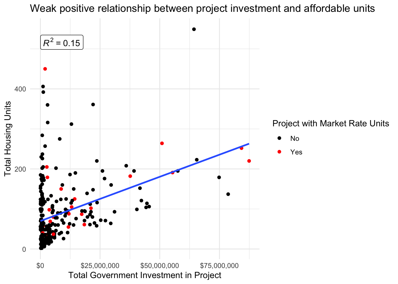
Given the limited local government funds available and the sizable need for housing in general, and affordable housing in particular, it is imperative that investments are made in a way that maximizes public benefit. Below I plot the relationship between government investment in a project and the total number of housing units produced. There is a weak positive relationship with significant variance between projects. These differences between projects deserves further research to determine the different factors that lead to a greater return for government investment.
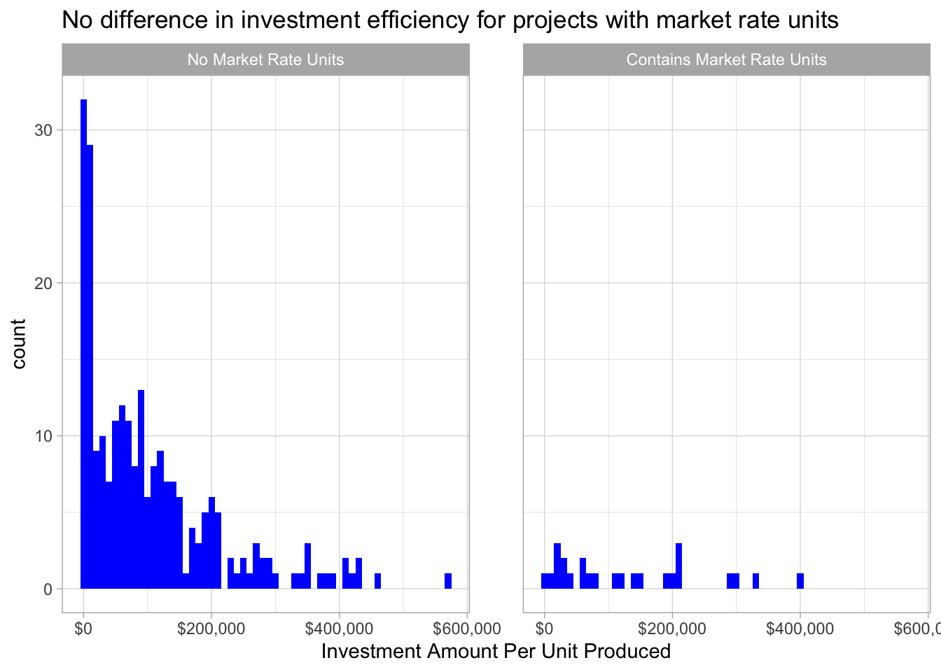
One possible variable that could contribute to a greater return for government investment is the presence of market rate housing in a project. These units could hypothetically offset some of the subsidy required by developers and thereby may necessitate less funding from the government. However, there were relatively few projects in the data sets examined that contained any market rate housing. This could be partly due to incomplete data as only one of the data sets used contained market rate unit data. Of the projects that did contain market rate units, they did not appear to differ significantly in the investment efficiency, calculated as the dollars of government investment per unit of affordable housing produced.
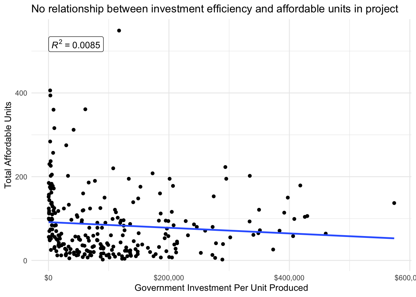
Similarly, we might expect that those projects with higher number of affordable housing units could require more investment per unit since these affordable units would require subsidy to offset the lower rents paid for them. Plotting the total affordable units in a project and the government investment per unit does not appear to show a relationship.
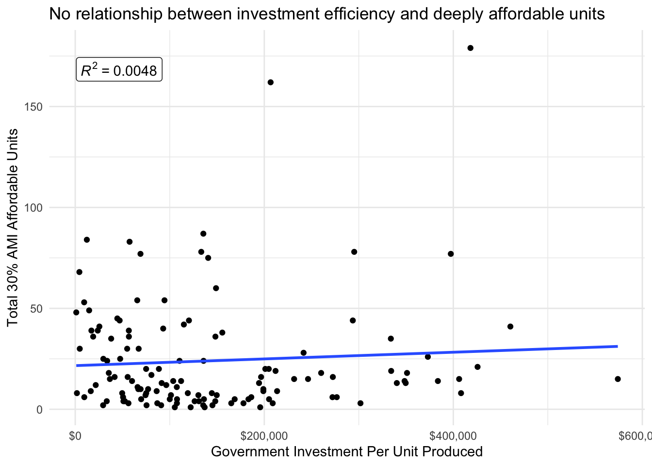
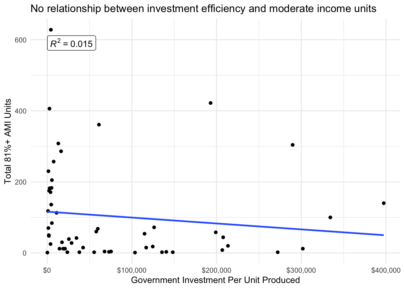
We also might expect that there would be relationships between different levels of affordability and the investment per unit produced. Affordable housing typically has income restrictions that are calculated based on the Area Median Income (AMI). For example some units that are considered “deeply” affordable housing are restricted to renters making below 30% AMI, while others are reserved for more moderate income renters making around 80% AMI. There does not appear to be a relationship between investment efficiency and either the number of deeply affordable housing units or moderately affordable housing units.
Mapping Affordable Housing Production
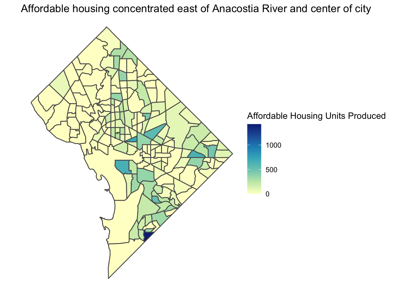
I use a third data set to map affordable housing production since 2015. As has been emphasized in previous research on housing in DC, new affordable housing construction has been concentrated in areas east of the Anacostia River and in the central part of DC. While many Census tracts have received some affordable housing production, there has been a notable lack of affordable housing production in areas west of Rock Creek Park.
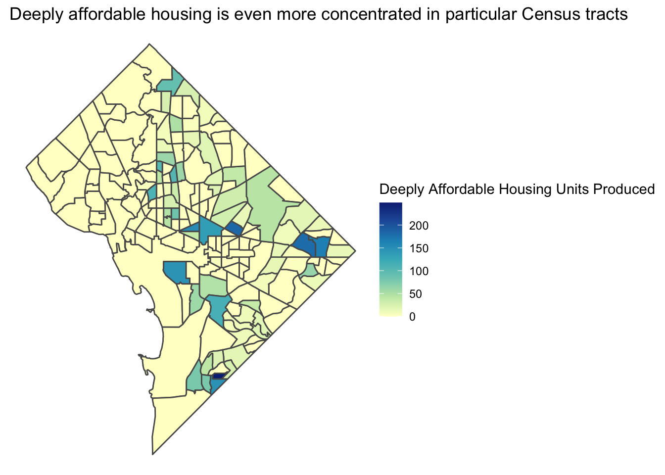
The distribution of deeply affordable housing (available to those making less than 30% AMI) is even more concentrated in particular Census tracts and less evenly spread throughout the city. This is likely due in part to the fact that many of these units are replacement units for public housing redevelopment projects, which are typically very large developments.
Predicting DC Government Investment by Project
I construct two machine learning models to predict the amount of DC government investment in a particular project. These include not just affordable housing projects, but other economic development investments including some related to small businesses, nonprofits, and arts and culture.
As part of the modeling process, feature engineering was conducted and largely based on recommendations and techniques from Bradley Boehmke & Brandon Greenwell (2020).
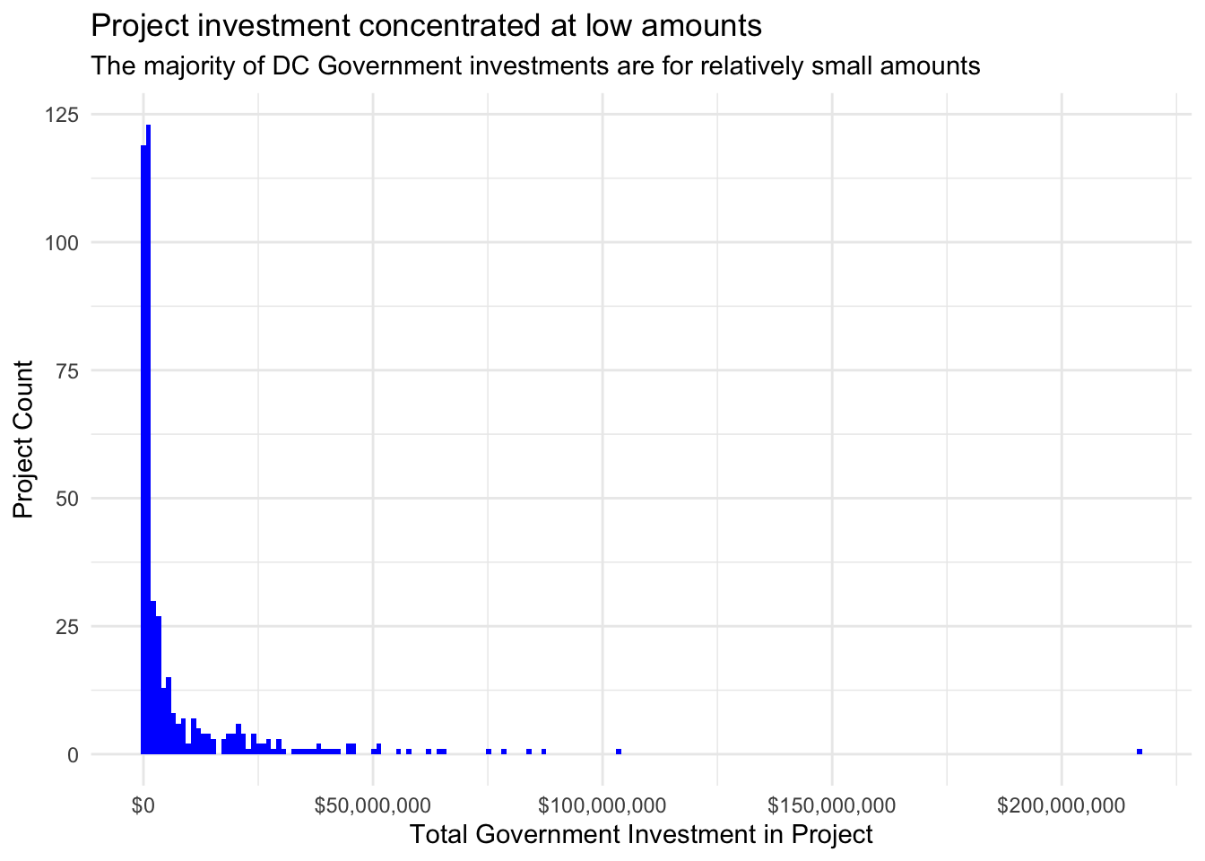
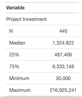
Notably, these investments are heavily right-skewed, with most investments under $1.5M and a long tail reaching a maximum of over $215M for one project. Due to this skew, I log-transform the project investment variable before building my predictive models. The stylized table below was produced by referencing a tutorial by Daniel D. Sjoberg, Michael Curry, Margie Hannum, Karissa Whiting, Emily C. Zabor (2020).
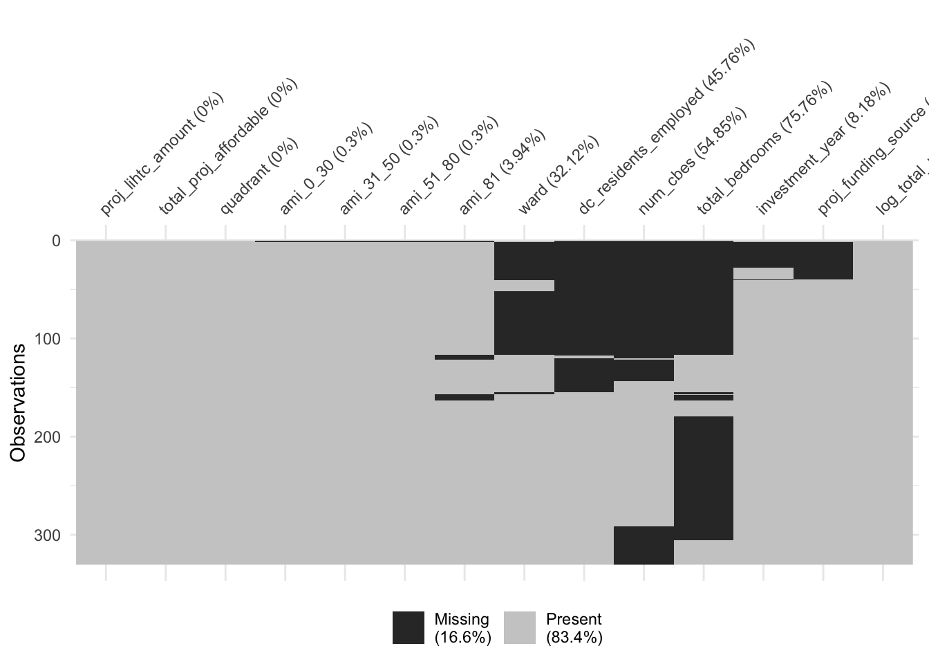
As can be seen in the below visualization of missing values across the data set, there were a number of variables that were contained in one data set but not the other, leading to projects that had missing values for these variables. These were imputed as part of the preprocessing steps.
I first train a K-Nearest Neighbor model, which outperforms a previous KNN model I conducted on just one of the data sets. These improvements are likely due to the additional data as well as additional preprocessing steps conducted. The root mean squared error term is not easily interpretable because it is in log-units, which will be reversed in a later step for further model evaluation.
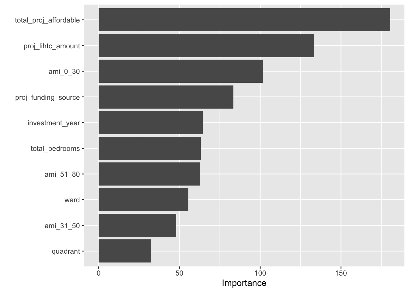
I then train a Random Forest model to predict project investment. The model implementation uses the tidymodels framework and was developed by referencing Bradley Boehmke & Brandon Greenwell (2020) and Hansjörg Plieninger (2020). This model performs better than the KNN model based on a lower RMSE value. I also visualize the variable importance for the RF model, which shows that total affordable housing units, amount of Low Income Housing Tax Credit investment, units at 30% AMI, and the project funding source play the most important roles in the model. While the initial visualizations appeared to show that there was not much of a relationship between investment and affordable units or deeply affordable units, this predictive model relied heavily on these two variables suggesting the possibility of some relationship.
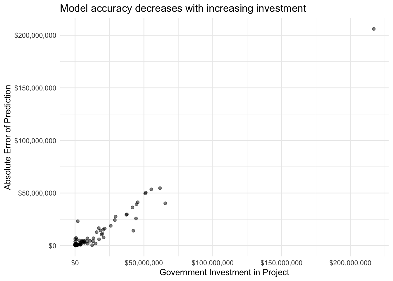
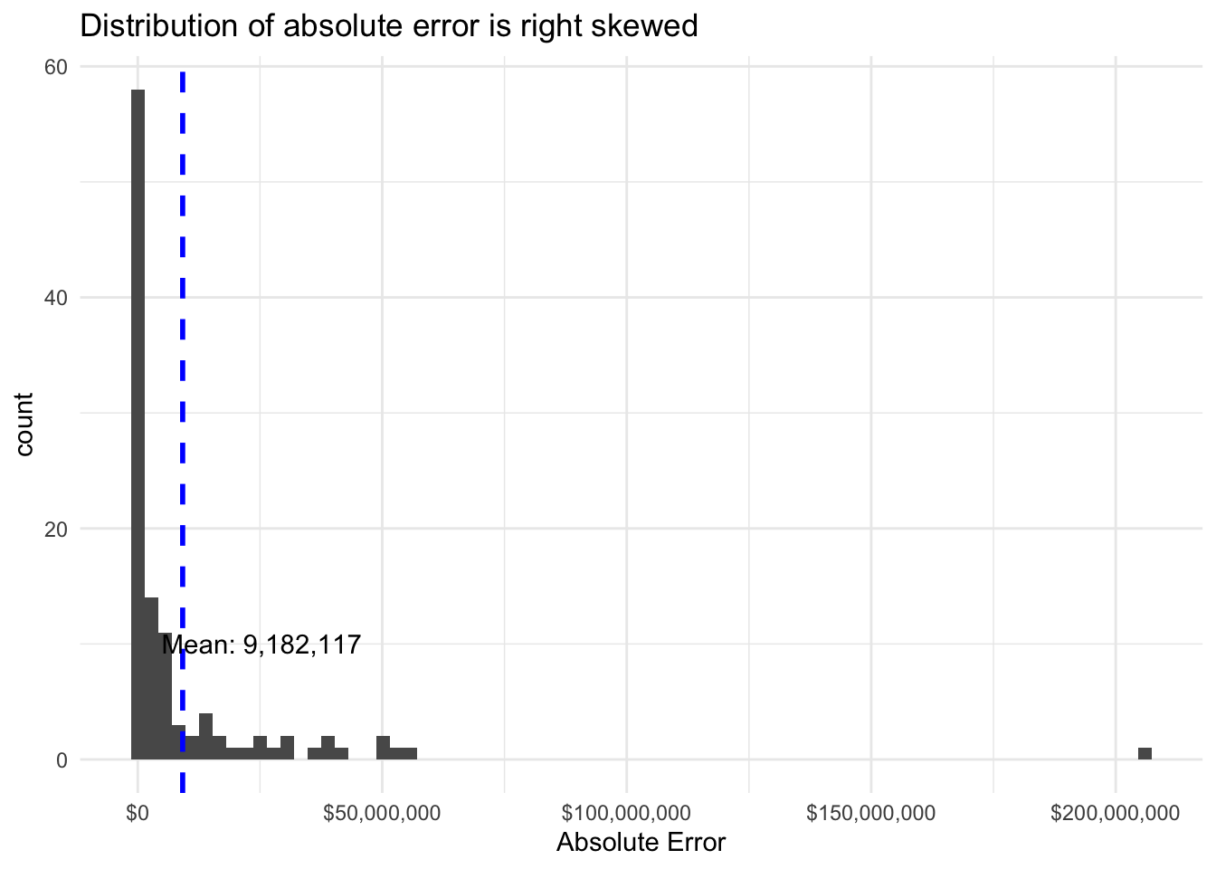
Finally, I use the identified best model to make predictions on the testing data set and then undo the log transformation to allow for further analysis. With a root mean squared error of $24,544,726 this model does not initially appear to perform very well considering that the vast majority of investments were well below this amount. Upon closer analysis, however, we see that the mean absolute error was much lower at $9,182,117. While still relatively high compared to most investments, this demonstrates the impact of outlier projects that were significantly larger than most other projects. This can be seen further by plotting the absolute error for individual projects against the actual investment and by considering the distribution of absolute error. We can see that for many project investment predictions there was relatively low error. Based on the composition of the data set, it makes sense that the model would perform better with the lower investment amounts.
Predicting Affordable Unit Production by Project
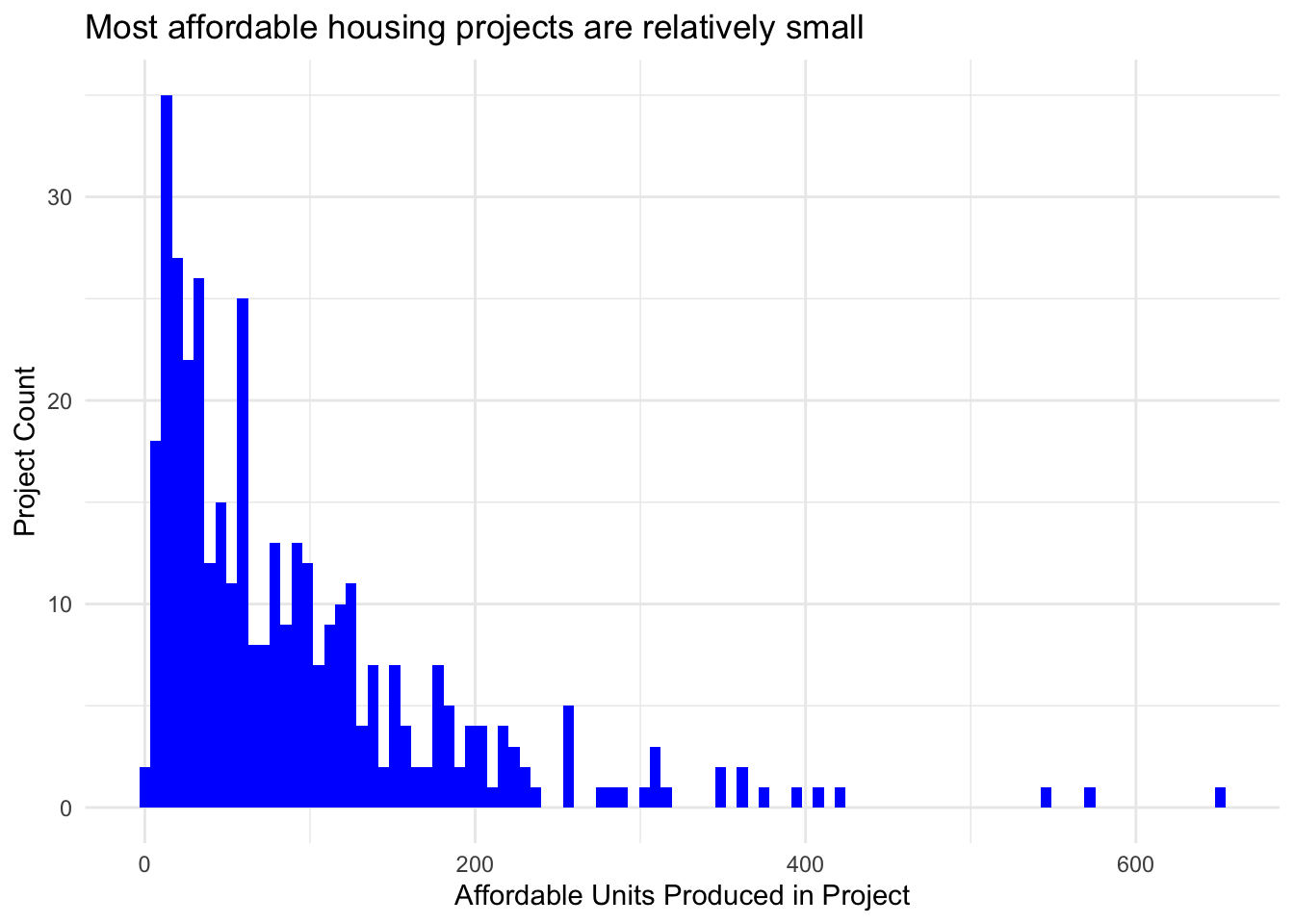
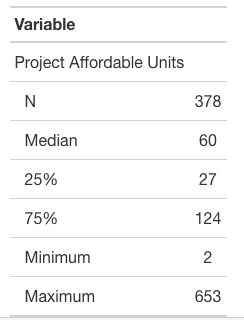
Similarly, I next produce a model to predict the number of affordable housing units produced by project. The number of affordable units per project is also right-skewed in the data with the majority of projects producing fewer than 60 units of affordable housing, but with a few producing over 500.
As with the previous model, feature engineering was conducted and largely based on recommendations and techniques from Bradley Boehmke & Brandon Greenwell (2020). The stylized table below was produced by referencing a tutorial by Daniel D. Sjoberg, Michael Curry, Margie Hannum, Karissa Whiting, Emily C. Zabor (2020).
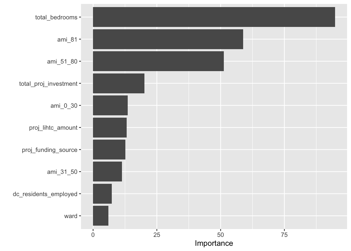
I first train multiple specifications of a K-Nearest Neighbor model. I then train a number of specifications of a Random Forest model, which signficantly outperforms the KNN model. Similarly, the model implementation uses the tidymodels framework and was developed by referencing Bradley Boehmke & Brandon Greenwell (2020) and Hansjörg Plieninger (2020). Again, the root mean squared error term is not initially meaningfully interpretable because of the log transformation of the outcome variable. Total bedroom, units at 81% AMI, and units at 51-80% AMI are the most important variables for the model. This is unsurprising as these all directly contribute to the total affordable units in a project or are very closely correlated.
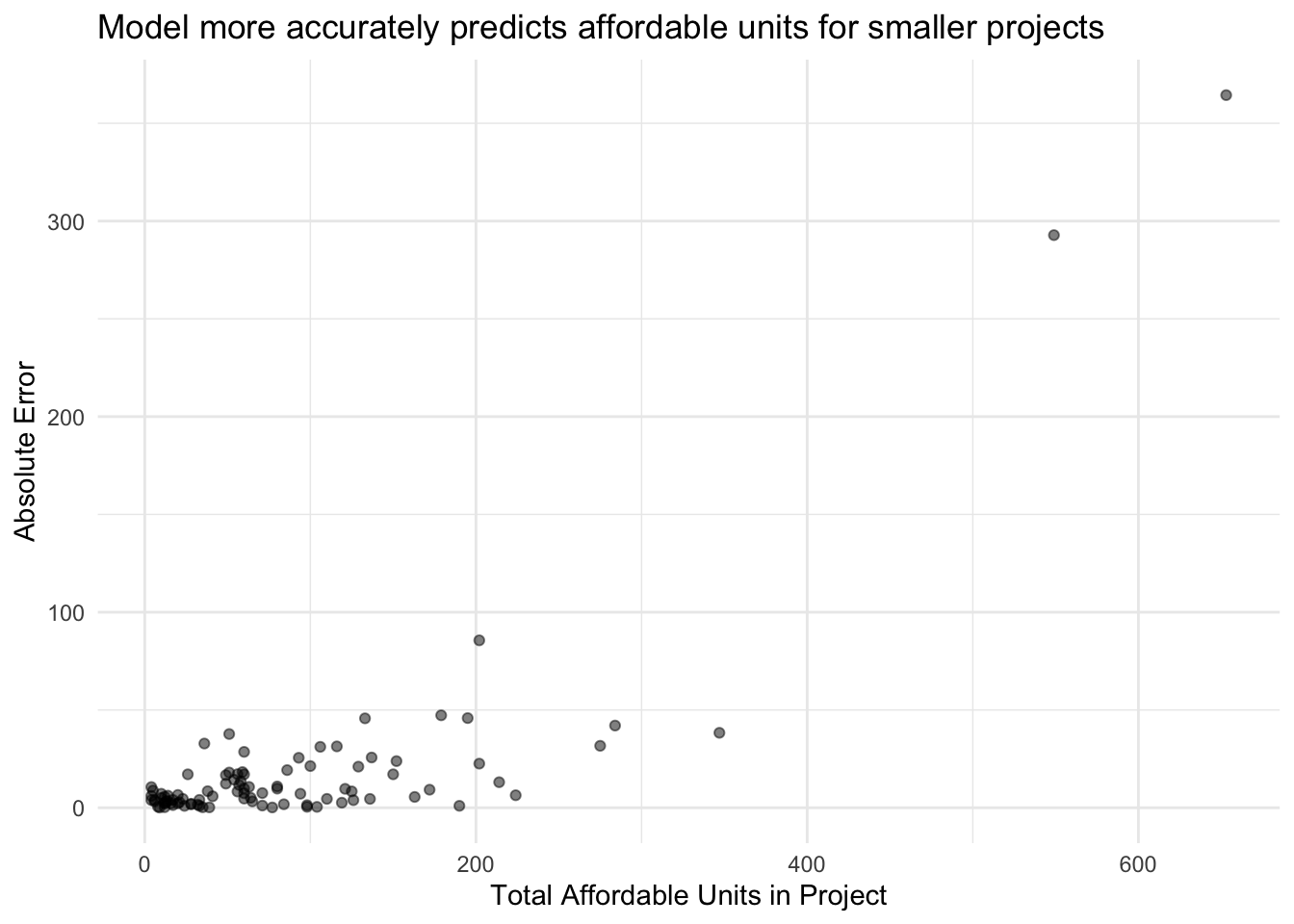
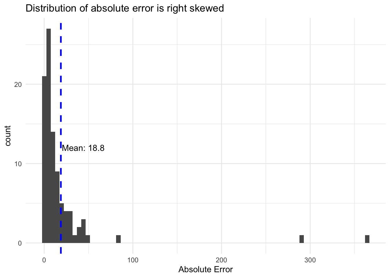
After selecting the optimal Random Forest model specification, I use this model to make predictions for the test data. After undoing the log transformation, the root mean squared error is approximately 51 units. This model performs better in comparison to the median than the model to predict investment in projects. Similarly, though, the mean absolute error is significantly lower with a value of approximately 19 units. This is a fairly good margin of error except for the smallest of projects.
The model does somewhat better at predicting projects in the middle of the distribution than the model for predicting investment. This is likely due to the fact that the affordable units per project were not as severely skewed as the investment per project. Overall, this model performs somewhat well and could be used as a way to flag particular projects that are proposed to produce a number of affordable units that are far outside the predictions of the model.
References
Bradley Boehmke & Brandon Greenwell. 2020. Hands-on Machine Learning with R. https://bradleyboehmke.github.io/HOML/index.html.
Daniel D. Sjoberg, Michael Curry, Margie Hannum, Karissa Whiting, Emily C. Zabor. 2020. http://www.danieldsjoberg.com/gtsummary/articles/tbl_summary.html.
Hansjörg Plieninger. 2020. Tutorial on Tidymodels for Machine Learning. https://hansjoerg.me/2020/02/09/tidymodels-for-machine-learning/.